Hello,
I modified the official example code plot_inv_2_dcip2d.py and used my own data to invert for resistivity and chargeability. The inversion results are not good, showing large areas of very high values. I tried adjusting the parameters, but the results did not improve. Could you please tell me what the main reason for this problem might be? Is it due to incorrect inversion parameter settings?
#%%
# %% Cell 1 - 导入所需模块
import warnings
from pathlib import Path
import matplotlib as mpl # 绘图基础模块
import matplotlib.pyplot as plt # 绘图库
import numpy as np
import pandas as pd
from discretize.utils import active_from_xyz
from discretize.utils import mkvc
from matplotlib.colors import LogNorm
from matplotlib.colors import Normalize
from matplotlib.ticker import ScalarFormatter
from pymatsolver.wrappers import UnusedArgumentWarning
from scipy.interpolate import griddata
from scipy.spatial import distance_matrix
from simpeg import data, optimization, inverse_problem, directives, inversion, maps, regularization, data_misfit
from simpeg.electromagnetics.static import induced_polarization as ip # IP模拟模块
from simpeg.electromagnetics.static import resistivity as dc
from simpeg.electromagnetics.static.utils import apparent_resistivity_from_voltage, plot_pseudosection
from simpeg.utils import get_default_solver
from build_2d_mesh import build_tensormesh, build_treemesh
solver = get_default_solver()
# ------------------------
# 1️⃣ 屏蔽警告
# ------------------------
warnings.filterwarnings('ignore', category=UnusedArgumentWarning)
warnings.filterwarnings('ignore', message="splu converted its input to CSC format")
# 设置绘图参数
plt.rcParams.update({'font.size': 12}) # 全局字体大小
mpl.rcParams['font.family'] = 'DejaVu Sans' # 字体类型
#%%
# %% Cell 2 设置数据源及相关参数
root = "F:/Earth/Geophysics/Induced Polarization/AGL_IP"
folder = "L_1_PD_Dip50m_AGL"
excel_file = f"{root}/{folder}/{folder}_Libreta_modify.xlsx"
sheet_name = "Hoja1"
chargeability_flag = "M2"
resistivity = "read"
drop_lower_zero = True
spacing = 50.0
# TensorMesh 适合平坦或轻微起伏的地形,实现简单;TreeMesh 适合复杂地形,更贴近真实情况
mesh_type = "tree"
use_log_conductivity = True
OUT_DIR = Path(f"{root}/inv_ip_2d_outputs") # 输出目录(脚本会创建)
OUT_DIR.mkdir(parents=True, exist_ok=True)
if not Path(excel_file).exists():
raise FileNotFoundError(f"指定的 Excel 文件不存在:{excel_file}")
print("读取 Excel:", excel_file)
df = pd.read_excel(excel_file, sheet_name=sheet_name)
# 删除缺失位置数据的行
df = df.dropna(subset=["A", "M", "N", "A_Z", "M_Z", "N_Z"])
# 向量化操作替代循环
if drop_lower_zero:
# 删除df中M1~M4小于0的行
df = df[(df[["M1(%)", "M2(%)", "M3(%)", "M4(%)"]] >= 0).all(axis=1)]
# 计算中间列
df["spacing_temp"] = df["N"] - df["M"]
df["n"] = (df["M"] - df["A"]) / spacing
# 验证电极间距
if not (df["spacing_temp"] == spacing).all():
invalid_rows = df[df["spacing_temp"] != spacing]
print(f"错误:发现{len(invalid_rows)}行电极间距不等于{spacing}")
print(invalid_rows[["A", "M", "N"]])
raise ValueError("电极间距不一致,请检查Excel文件")
threshold = 1e-2 # 1 cm
for name1 in ["A", "M", "N"]:
for name2 in ["A", "M", "N"]:
if name1 >= name2: # 避免重复对比
continue
coords1 = df[[name1, f"{name1}_Z"]].values
coords2 = df[[name2, f"{name2}_Z"]].values
dists = np.linalg.norm(coords1 - coords2, axis=1)
print(f"{name1}-{name2} 最小距离: {dists.min():.6f} m")
#%%
# %% Cell 3 - 读取二维地形文件
topo_df = df.dropna(subset=["Metro", "Z"])
metro_min, metro_max = df["Metro"].min(), df["Metro"].max()
topo_2d = topo_df[["Metro", "Z"]].to_numpy()
#%%
# %% Cell 4 - 绘制地形
#%%
# %% Cell 5 - 读取极化率观测数据
# 向量化计算视电阻率
if resistivity == "read":
AM = df["M"] - df["A"]
AN = df["N"] - df["A"]
k = 2 * np.pi * (AM * AN) / (AN - AM)
# Normalized voltage measurements[V / A]
df["volt"] = df["VP(mv)"] / df["Amp (mA)"]
df["resistivity"] = k * df["volt"]
else:
df["resistivity"] = resistivity
# apparent_resistivity = df["resistivity"].to_numpy()
volt = df["volt"].to_numpy()
# 向量化计算视极化率
if chargeability_flag == "Mean":
df["chargeability"] = df[["M1(%)", "M2(%)", "M3(%)", "M4(%)"]].mean(axis=1)
else:
df["chargeability"] = df[f"{chargeability_flag}(%)"]
# % 转换为 V/V
apparent_chargeability = df["chargeability"].to_numpy() / 100.0
dc_sources, ip_sources = [], []
# 先提取成 NumPy 数组,减少 pandas 开销
cols = ["A", "A_Z", "M", "M_Z", "N", "N_Z"]
A, A_Z, M, M_Z, N, N_Z = (df[c].to_numpy() for c in cols)
# 用纯 NumPy 数组迭代(非常快)
for a, az, m, mz, n, nz in zip(A, A_Z, M, M_Z, N, N_Z):
m_pos = np.array([m, mz])
n_pos = np.array([n, nz])
a_pos = np.array([a, az])
dc_rx = dc.receivers.Dipole(m_pos, n_pos, data_type="volt")
ip_rx = ip.receivers.Dipole(m_pos, n_pos, data_type="apparent_chargeability")
dc_sources.append(dc.sources.Pole([dc_rx], a_pos))
ip_sources.append(ip.sources.Pole([ip_rx], a_pos))
# 创建测量对象
dc_survey = dc.survey.Survey(dc_sources)
dc_data = data.Data(dc_survey, dobs=volt)
ip_survey = ip.survey.Survey(ip_sources)
ip_data = data.Data(ip_survey, dobs=apparent_chargeability)
#%%
# %% Cell 6 - 绘制视极化率假剖面
# 在 fwd_ip_2d_user.py 中实现
# %config InlineBackend.figure_format = 'retina'
apparent_resistivity = apparent_resistivity_from_voltage(
dc_data.survey, dc_data.dobs
)
apparent_conductivity = 1 / apparent_resistivity
# Plot apparent conductivity pseudo-section
fig = plt.figure(figsize=(18, 4))
ax1 = plt.subplot(111)
# ax1 = fig.add_axes([0.1, 0.15, 0.75, 0.78])
plot_pseudosection(
dc_data.survey,
apparent_resistivity,
"contourf",
ax=ax1,
scale="log",
cbar_label=r"$\rho$ (Ohm·m)",
mask_topography=True,
contourf_opts={"levels": 20, "cmap": mpl.cm.jet},
)
ax1.set_title("Apparent Resistivity")
plt.show()
fig = plt.figure(figsize=(18, 4))
ax1 = plt.subplot(111)
plot_pseudosection(
dc_data.survey,
apparent_conductivity,
"contourf",
ax=ax1,
scale="log",
cbar_label="S/m",
mask_topography=True,
contourf_opts={"levels": 20, "cmap": mpl.cm.jet},
)
ax1.set_title("Apparent Conductivity")
plt.show()
# Plot apparent chargeability in pseudo-section
apparent_chargeability = ip_data.dobs
fig = plt.figure(figsize=(18, 4))
ax1 = plt.subplot(111)
plot_pseudosection(
ip_data.survey,
apparent_chargeability,
"contourf",
ax=ax1,
scale="linear",
cbar_label="V/V",
mask_topography=True,
contourf_opts={"levels": 20, "cmap": mpl.cm.jet},
)
ax1.set_title("Apparent Chargeability")
plt.show()
#%%
# %% Cell 7 - 设置观测数据标准差
# 检查数据范围
print(f"归一化电压数据范围:{np.min(dc_data.dobs)} - {np.max(dc_data.dobs)}")
relative_error = 0.05 # 相对误差5%
std_original_dc_data = relative_error*np.abs(dc_data.dobs)
print(f"原始数据 {int(relative_error*100)}% 标准差范围:{np.min(std_original_dc_data)} - {np.max(std_original_dc_data)}")
absolute_error_floor = np.percentile(np.abs(dc_data.dobs), 5) * 0.01 # 绝对下限
print(f"归一化电压误差下限设置为:{absolute_error_floor}")
dc_data.standard_deviation = np.maximum(std_original_dc_data, absolute_error_floor)
print(f"归一化电压标准差范围:{np.min(dc_data.standard_deviation)} - {np.max(dc_data.standard_deviation)}")
# %% Cell 8 - 构建 Mesh 网格
dh = spacing / 5 # 基础网格单元尺寸
dom_width_x = 2000 # 水平方向区域宽度
dom_width_z = 1000 # 垂直方向区域深度
# print(f"区域宽度:{dom_width_x},区域深度:{dom_width_z}")
# pad_x扩展网格,+dh/2防止电极与网格节点重合
if mesh_type == "tree":
# 创建 TreeMesh 网格
z_min, z_max = topo_df["Z"].max() - 300, topo_df["Z"].max()
xp, zp = np.meshgrid([metro_min, metro_max], [z_min, z_max])
box_bound = np.c_[mkvc(xp), mkvc(zp)]
mesh = build_treemesh(topography_2d=topo_2d, electrodes_2d=topo_2d,
width_x=dom_width_x, width_z=dom_width_z, dh0=dh,
refine_surface_levels=[0, 0, 4, 4],
refine_points_levels=[4, 4],
refine_box_levels=[0, 0, 2, 8],
box_bounding=box_bound,
pad_x=0.1) # 地形+电极+区域细化
elif mesh_type == "tensor":
# 创建 TensorMesh 网格
mesh = build_tensormesh(electrodes_2d=topo_2d, width_x=dom_width_x, width_z=dom_width_z, dh0=dh, pad_x=0.1)
# %% Cell 9 - 定义活动单元
ind_active = active_from_xyz(mesh, topo_2d)
elec_locs = dc_data.survey.unique_electrode_locations # 所有电极坐标
#%%
# %% Cell 10 - 将电极投影到地形表面
# 调整电极位置匹配实际地形,消除地形引起的假异常
dc_data.survey.drape_electrodes_on_topography(mesh, ind_active, topo_cell_cutoff="top")
ip_data.survey.drape_electrodes_on_topography(mesh, ind_active, topo_cell_cutoff="top")
# 计算几何因子
dc_survey.set_geometric_factor()
ip_survey.set_geometric_factor()
elec_locs = dc_data.survey.unique_electrode_locations # 所有电极坐标
print(f"{'='*20} 电极位置调整后 {'='*20}")
# 判断电极位置是否与网格重合
mesh_nodes = mesh.nodes
for i, loc in enumerate(elec_locs):
dists = np.min(np.linalg.norm(mesh_nodes - loc, axis=1))
print(f"电极 {i} 位置为 {loc} 距网格节点 {dists:.4f} m", end="")
if dists < 1e-12:
print(f",电极 {i} 与网格节点重合")
else:
print("")
#%%
# %% Cell 11 - 定义电导率参数
# 定义电导率值 (单位: S/m),建立典型地质体的电性参数库
# 空气电导率 (极低)
air_conductivity = 1e-8
# 背景介质电导率
background_conductivity = 1e-2
# background_conductivity = np.exp(np.mean(np.log(apparent_conductivity)))
print(f"设置背景电导率值为 {background_conductivity} S/m")
# %% Cell 13 - 定义映射
# 将活动单元的电导率映射到整个网格,活动单元保持原值,非活动单元(空气)设为1e-8 S/m,用于正演模拟计算
active_map = maps.InjectActiveCells(mesh, ind_active, air_conductivity)
# 统计活动单元数量
nC = int(ind_active.sum())
if use_log_conductivity:
# 把「log空间的模型参数」转换为「线性空间的电导率」,用于模型正演
conductivity_map = active_map * maps.ExpMap()
starting_conductivity_model = np.log(background_conductivity) * np.ones(nC)
# upper 对应 0.2 Ω·m,lower 对应 1000 Ω·m
sigma_lower, sigma_upper = np.log(1e-3), np.log(5)
else:
conductivity_map = active_map
starting_conductivity_model = background_conductivity * np.ones(nC)
sigma_lower, sigma_upper = 1e-3, 5
# 构建 DC 正演算子(用于反演 sigma)
# survey 观测系统(测线、极对位置),定义电流注入点和电位测量点
# sigmaMap 电导率映射,把反演模型 m 转换为网格上完整的电导率场
# 用 log(σ) 空间做反演,反演过程中模型变化时自动转换到 σ 空间进行正演
# storeJ 是否缓存灵敏度矩阵 J(Jacobian)设置为 True 可以加快反演多次求导的速度,但会占内存;
dc_simulation = dc.Simulation2DNodal(
mesh, survey=dc_data.survey, sigmaMap=conductivity_map, storeJ=True, solver=solver,
)
dc_data_misfit = data_misfit.L2DataMisfit(data=dc_data, simulation=dc_simulation)
dc_regularization = regularization.WeightedLeastSquares(
mesh,
active_cells=ind_active,
reference_model=starting_conductivity_model,
alpha_s=0.01,
alpha_x=1,
alpha_y=1,
)
# maxIter 允许优化器最多进行的外层迭代次数,相当于反演的最大步数,达到这个次数会强制停止。
# lower, upper 模型参数的硬边界,如果超出这个范围,会被投影回范围内。
# maxIterLS 线搜索最大步长尝试次数,每次外层迭代中,算法要尝试不同的步长找到能降低目标函数的更新方向。
# 如果连续 maxIterLS 次都找不到合适步长,就会报错 linesearch got broken.
# 🔹 调大可以避免“刚开始卡住”的问题
# 🔹 调小可以加速反演(但可能不收敛)
# cg_maxiter (maxIterCG) 内层共轭梯度解算器的最大迭代次数。每次外层迭代中,需要解一个二阶近似的线性方程组 CG 用于求解。
# CG 不是直接解精确解,而是迭代逼近 → 这里限制最多 10 步。
# 🔹 如果模型单元很多( > 10⁴),可以调大到 20–50
# 🔹 初期调小(5–10)可以加速调试
# cg_atol (tolCG) = 1e-3,内层CG解算器的收敛容差。当残差 < 1e-3 时认为 CG 已经收敛,不再继续迭代。
# 🔹 较小(1e-4~1e-5) → 解更精确但更慢
# 🔹 较大(1e-2) → 解更快但不太精确
# tolF 函数值变化容差
# 在一次外层迭代中,先完成所有 CG 迭代,得到一个整体更新方向 p,然后才执行一次线搜索决定步长 α
# Step 1: 构造Gauss-Newton Hessian
# Step 2: 用CG解 Hessian * p = -grad ,最多 cg_maxiter 次 or 残差 < cg_atol
# Step 3: 沿着 p 方向做线搜索,最多尝试 maxIterLS 个步长
# Step 4: 更新模型 m = m + α * p
dc_optimization = optimization.ProjectedGNCG(
maxIter=80, lower=sigma_lower, upper=sigma_upper, maxIterLS=60, cg_maxiter=50, tolF=1e-8, cg_atol=1e-4)
# dc_optimization = optimization.InexactGaussNewton(
# maxIter=60, maxIterLS=50, cg_maxiter=50, cg_atol=1e-3)
dc_inverse_problem = inverse_problem.BaseInvProblem(
dc_data_misfit, dc_regularization, dc_optimization
)
# 根据每个单元对数据的“敏感度”自动调整正则化权重,让有数据约束的单元更“自由”,没数据约束的单元被更强烈抑制
# threshold 很小(接近 0)
# 结果:低敏感区权重 → 非常大 → 这些单元几乎不能离开参考模型(非常强的抑制)。
# 优点:能有效抑制无约束区的虚假异常(稳定)。
# 缺点:设置过小,整个反演可能被“僵化”——优化器难以在这些区域做任何有意义的改变,可能导致线搜索失败(linesearch got broken)或迭代停滞。此外若敏感度计算噪声较大,会被极端值主导。
# threshold 较大
# 结果:权重不会爆炸,正则化在低敏感区不那么强。
# 优点:允许这些区域有更多自由度;如果你确实怀疑低敏感区可能有真实异常(或参考模型不可靠),这样可能更好。
# 缺点:会增加在无约束区出现伪差或噪声的风险(因为正则化不够强)。
update_sensitivity_weighting = directives.UpdateSensitivityWeights(every_iteration=True, threshold_value=1e-2)
# 在 SimPEG 的反演中,会同时考虑数据失配项和模型正则化项:𝜙(𝑚)=𝜙𝑑(𝑚)+𝛽𝜙𝑚(𝑚)
# 𝜙𝑑(𝑚),衡量模拟数据和实测数据的差异。𝜙𝑚(𝑚),限制模型的复杂度,避免过拟合
# 初始 𝛽 值估计器,它通过雅可比矩阵与正则化算子之间的特征值比值 来估计 𝛽 的合适初值。
# 𝛽 数值大,初期强平滑,更稳、更慢;数值小,初期更快拟合数据,但有可能不稳或不物理。
starting_beta = directives.BetaEstimate_ByEig(beta0_ratio=1e1)
# 冷却策略,从一个非常平滑的初始模型逐步演化为更复杂的模型,防止直接过拟合噪声。
# coolingFactor,每次冷却时 𝛽 除以这个因子(即减小的倍数)
# coolingRate 每隔多少次迭代冷却一次
# coolingRate=1(线性最小二乘问题),完全线性的问题,Jacobian 矩阵恒定不变
# coolingRate=2(弱非线性问题),大多数地球物理反演问题,包括用户正在处理的电阻率/IP反演
# coolingRate=3(强非线性问题),高度非线性问题,优化地形复杂,容易陷入局部极小值
beta_schedule = directives.BetaSchedule(coolingFactor=3, coolingRate=2)
# 是否将每次迭代的目标函数值(phi_d, phi_m, beta等)额外保存为 .txt 文本文件。默认 False,表示只在内存中记录。
save_iteration = directives.SaveOutputEveryIteration(on_disk=False)
# 当数据失配项 𝜙𝑑 拟合到误差水平(𝜒=1)时就提前终止反演,防止继续迭代造成过拟合。
# 理论上,如果误差估计合理,且模型恰好拟合到误差水平:𝜙𝑑≈𝑁(𝑁=数据点数),SimPEG 会计算当前反演模型的 chi 值:𝜒=𝜙𝑑/𝑁
# chifact=1 → 目标:𝜒≈1,即数据拟合到误差水平(常用)
# chifact<1 → 目标比误差还小,可能会过拟合
# chifact>1 → 允许比误差大一些,能更快停止但精度低
target_misfit = directives.TargetMisfit(chifact=1)
# 在反演过程中定期更新雅可比矩阵(Jacobian)的预条件子,从而加快共轭梯度(CG)求解速度、提高数值稳定性
update_jacobi = directives.UpdatePreconditioner()
directives_list = [
update_sensitivity_weighting,
starting_beta,
beta_schedule,
save_iteration,
target_misfit,
update_jacobi,
]
dc_inversion = inversion.BaseInversion(
dc_inverse_problem, directiveList=directives_list
)
recovered_conductivity_model = dc_inversion.run(starting_conductivity_model)
#%%
# %% Cell 14 - 绘图专用映射
# 可视化专用映射,活动单元保持原值,非活动单元设为NaN,避免空气区域干扰地下结构显示
plotting_map = maps.InjectActiveCells(mesh, ind_active, np.nan)
# 诊断 2: 反演后(或每次迭代保存 dpred 后)查看残差分布
dpred_dc = dc_inverse_problem.dpred
print(f"dc pred min: {np.min(dpred_dc)}, max: {np.max(dpred_dc)}")
resid_dc = (dc_data.dobs - dpred_dc) / dc_data.standard_deviation
print("resid stats: ", np.percentile(resid_dc, [0,1,5,25,50,75,95,99,100]))
# 打印最大的几个残差点索引
big_idx = np.argsort(np.abs(resid_dc))[-10:][::-1]
print("top 10 largest residuals (idx, resid, obs, pred, std):")
for i in big_idx:
print(i, resid_dc[i], dc_data.dobs[i], dpred_dc[i], dc_data.standard_deviation[i])
# Plot
fig = plt.figure(figsize=(18, 12))
data_array = [np.abs(dc_data.dobs), np.abs(dpred_dc), resid_dc]
plot_title = ["Observed", "Predicted", "Normalized Misfit"]
plot_units = ["S/m", "S/m", ""]
scale = ["log", "log", "linear"]
ax1 = 3 * [None]
cax1 = 3 * [None]
cbar = 3 * [None]
cplot = 3 * [None]
for ii in range(0, 3):
ax1[ii] = fig.add_axes([0.1, 0.70 - 0.31 * ii, 0.7, 0.23])
cax1[ii] = fig.add_axes([0.81, 0.70 - 0.31 * ii, 0.02, 0.23])
cplot[ii] = plot_pseudosection(
dc_data.survey,
data_array[ii],
"contourf",
ax=ax1[ii],
cax=cax1[ii],
scale=scale[ii],
cbar_label=plot_units[ii],
mask_topography=True,
contourf_opts={"levels": 25, "cmap": mpl.cm.viridis},
)
ax1[ii].set_title(plot_title[ii])
plt.show()
#%%
# %% Cell 15 - 绘制电阻率模型
if use_log_conductivity:
resistivity_lower = 1 / np.exp(sigma_upper)
resistivity_upper = 1 / np.exp(sigma_lower)
else:
resistivity_lower = 1 / sigma_lower
resistivity_upper = 1 / sigma_upper
print(f"反演模型设定电阻率范围为 {resistivity_lower:.2f}~{resistivity_upper:.2f} Ohm·m")
norm = LogNorm(vmin=resistivity_lower, vmax=resistivity_upper)
# 通过映射将模型参数转换为实际电导率值,使用对数反演时conductivity_map=active_map * maps.ExpMap()
recovered_conductivity = conductivity_map * recovered_conductivity_model
recovered_conductivity[~ind_active] = np.nan
recovered_resistivity = 1.0 / recovered_conductivity
print(f"反演得到的电阻率模型范围为 {np.nanmin(recovered_resistivity):.2f}~{np.nanmax(recovered_resistivity):.2f} Ohm·m")
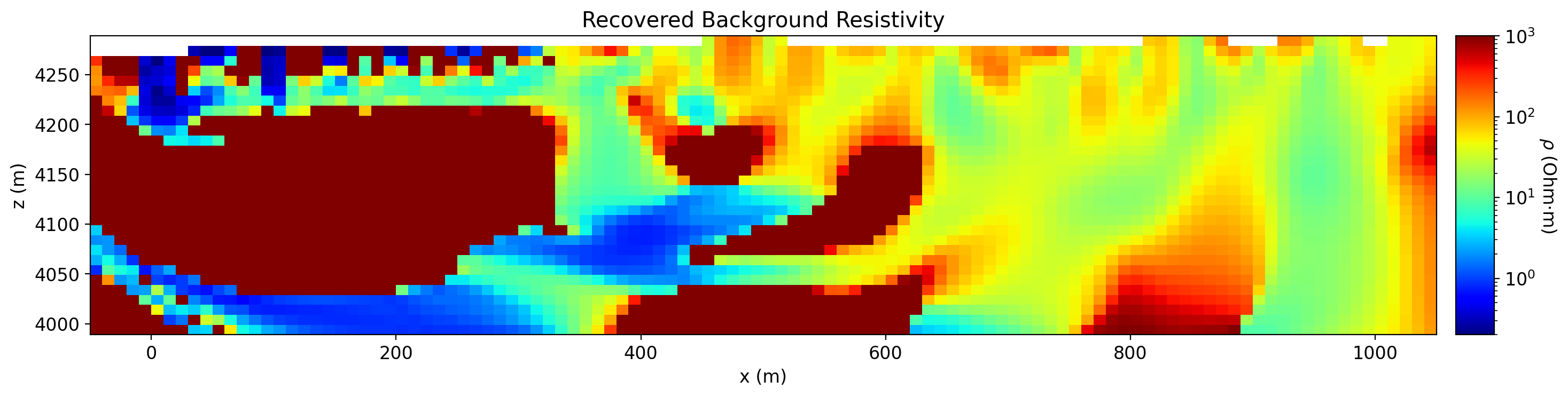
fig = plt.figure(figsize=(18, 4))
ax1 = fig.add_axes([0.1, 0.1, 0.7, 0.7])
# RdYlBu_r颜色映射
mesh.plot_image(
recovered_resistivity,
ax=ax1,
grid=False,
pcolor_opts={"norm": norm, "cmap": mpl.cm.jet},
)
ax1.set_xlim(metro_min, metro_max)
ax1.set_ylim(topo_df["Z"].max() - 300, topo_df["Z"].max())
ax1.set_title("Recovered Background Resistivity")
ax1.set_xlabel("x (m)")
ax1.set_ylabel("z (m)")
ax2 = fig.add_axes([0.81, 0.1, 0.02, 0.7])
cbar = mpl.colorbar.ColorbarBase(ax2, norm=norm, orientation="vertical", cmap=mpl.cm.jet)
cbar.set_label(r"$\rho$ (Ohm·m)", rotation=270, labelpad=15, size=12)
plt.show()
#%%
# %% Cell 15 - 绘制电阻率模型的等值线剖面图
# 提取活动单元数据
active_resistivity = recovered_resistivity[ind_active]
active_centers = mesh.cell_centers[ind_active]
# 确定绘图范围
# x_min, x_max = np.min(active_centers[:, 0]), np.max(active_centers[:, 0])
x_min, x_max = metro_min, metro_max
z_min, z_max = topo_df["Z"].max() - 300, topo_df["Z"].max()
print(f"绘制的等值线剖面范围:{x_min:.2f}~{x_max:.2f} m, {z_min:.2f}~{z_max:.2f} m")
# 创建精细规则网格
grid_x, grid_z = np.mgrid[
x_min:x_max:(x_max-x_min) * 2j, # 点沿x方向
z_min:z_max:(z_max-z_min) * 2j # 点沿z方向
]
# 线性插值
grid_resistivity = griddata(
active_centers[:, :2], # 输入点坐标 (x, z)
active_resistivity, # 输入点值
(grid_x, grid_z), # 输出网格
method='linear', # 线性插值
fill_value=np.nan # 边界外设为NaN
)
fig, ax = plt.subplots(figsize=(18, 4))
# 1. 计算等值线层级(对数空间均匀分布)
log_min = np.log10(resistivity_lower)
log_max = np.log10(resistivity_upper)
# 创建等值线填充图
contour_fill = ax.contourf(
grid_x, grid_z, grid_resistivity,
levels=np.logspace(log_min, log_max, 50),
cmap='jet',
norm=LogNorm(),
alpha=0.8
)
# 添加等值线
contour_lines = ax.contour(
grid_x, grid_z, grid_resistivity,
levels=np.logspace(log_min, log_max, 10),
colors='k',
linewidths=0.5
)
# 在等值线上显示数值
ax.clabel(
contour_lines,
inline=True,
fontsize=10,
fmt='%.0f', # 整数格式
colors='black' # 黑色文字
)
# 添加地形
ax.plot(topo_2d[:, 0], topo_2d[:, 1], 'k-', linewidth=2)
# 添加电极位置
electrode_x = dc_data.survey.unique_electrode_locations[:, 0]
electrode_z = dc_data.survey.unique_electrode_locations[:, 1]
ax.scatter(electrode_x, electrode_z, s=30, c='k', marker='v', label='Electrodes')
# 设置坐标轴
ax.set_xlim(x_min, x_max)
ax.set_ylim(z_min, z_max)
# ax.invert_yaxis() # 深度向下为正
ax.set_xlabel('Distance (m)')
ax.set_ylabel('Elevation (m)')
ax.set_title('Resistivity Section (Contoured)')
# 添加颜色条
cbar = fig.colorbar(contour_fill, ax=ax)
cbar.set_label('Resistivity (Ω·m)')
levels = np.logspace(log_min, log_max, 10)
cbar.set_ticks(levels)
formatter = ScalarFormatter(useMathText=False)
formatter.set_scientific(False) # 不使用科学计数法
formatter.set_useLocale(False)
cbar.ax.yaxis.set_major_formatter(formatter)
plt.tight_layout()
plt.show()
#%%
fig, ax = plt.subplots(figsize=(18, 4))
# 先把数据裁剪在指定范围
grid_resistivity = np.clip(grid_resistivity, resistivity_lower, 120)
# 1. 计算等值线层级(线性空间均匀分布)更新上下限为裁剪后的真实范围
lin_min = np.nanmin(grid_resistivity)
lin_max = np.nanmax(grid_resistivity)
print(f"绘图数据范围为:{lin_min}~{lin_max}Ω")
# 创建等值线填充图
contour_fill = ax.contourf(
grid_x, grid_z, grid_resistivity,
levels=np.linspace(lin_min, lin_max, 50),
cmap='jet',
alpha=0.8
)
# 添加等值线
contour_lines = ax.contour(
grid_x, grid_z, grid_resistivity,
levels=np.linspace(lin_min, lin_max, 10),
colors='k',
linewidths=0.5
)
# 在等值线上显示数值
ax.clabel(
contour_lines,
inline=True,
fontsize=10,
fmt='%.0f', # 整数格式
colors='black' # 黑色文字
)
# 添加地形
ax.plot(topo_2d[:, 0], topo_2d[:, 1], 'k-', linewidth=2)
# 添加电极位置
electrode_x = dc_data.survey.unique_electrode_locations[:, 0]
electrode_z = dc_data.survey.unique_electrode_locations[:, 1]
ax.scatter(electrode_x, electrode_z, s=30, c='k', marker='v', label='Electrodes')
# 设置坐标轴
ax.set_xlim(x_min, x_max)
ax.set_ylim(z_min, z_max)
# ax.invert_yaxis() # 深度向下为正
ax.set_xlabel('Distance (m)')
ax.set_ylabel('Elevation (m)')
ax.set_title('Resistivity Section (Contoured)')
# 添加颜色条
cbar = fig.colorbar(contour_fill, ax=ax)
cbar.set_label('Resistivity (Ω·m)')
levels = np.linspace(lin_min, lin_max, 10)
cbar.set_ticks(levels)
formatter = ScalarFormatter(useMathText=False)
formatter.set_scientific(False) # 不使用科学计数法
formatter.set_useLocale(False)
cbar.ax.yaxis.set_major_formatter(formatter)
plt.tight_layout()
plt.show()
#%%
# %% Cell 16 - 定义极化率映射
# 检查数据范围
print(f"视极化率数据范围:{np.min(ip_data.dobs)} - {np.max(ip_data.dobs)}")
std_original_ip_data = 0.05 * np.abs(ip_data.dobs)
print(f"原始数据 5% 标准差范围:{np.min(std_original_ip_data)} - {np.max(std_original_ip_data)}")
ip_std_floor = max(5e-3, 0.01 * np.median(np.abs(ip_data.dobs))) # 绝对下限
print(f"视极化率误差下限设置为:{ip_std_floor}")
# 每个观测值误差为其绝对值的 5%,更符合实际测量误差,电阻率大值对应的误差更大,设置标准差下限
ip_data.standard_deviation = np.maximum(std_original_ip_data, ip_std_floor)
# 检查标准差
print(f"视极化率标准差范围: {np.min(ip_data.standard_deviation)} - {np.max(ip_data.standard_deviation)}")
air_chargeability = 0.0
background_chargeability = 1e-6
# 创建一个map对象,设置网格里哪些单元是真正参与反演的活动单元,非活动单元用第三个参数的值填充(0.0)
active_map = maps.InjectActiveCells(mesh, ind_active, air_chargeability)
nC = int(ind_active.sum())
chargeability_map = active_map
# %% Cell 17 - 定义初始与参考极化率模型
# 构造初始极化率模型(长度等于活动单元数 n_active),每个单元初始值为 1e-6(很小的正值,作为反演的起点)。
starting_chargeability_model = background_chargeability * np.ones(nC)
reference_chargeability_model = np.zeros_like(starting_chargeability_model)
#%%
# %% Cell 18 - 定义 L2 反演的正演算子
# sigma 电导率(作为正演中电场求解的 sigma);将对数模型转换为实际电导率
# etaMap 极化率(chargeability)的映射,即把 n_active 尺寸的极化率模型注入到网格。
# storeJ 在正演过程中保存雅可比矩阵(Jacobian),便于反演重复使用以加速运算。
ip_simulation = ip.Simulation2DNodal(
mesh,
survey=ip_data.survey,
etaMap=chargeability_map,
sigma=conductivity_map * recovered_conductivity_model,
storeJ=True,
solver=solver,
)
# %% Cell 19 - 数据失配项
ip_data_misfit = data_misfit.L2DataMisfit(data=ip_data, simulation=ip_simulation)
# %% Cell 20 - 正则化项
# 构造正则化决定了反演模型要有多“平滑”、多接近参考模型”
# active_cells 标记哪些单元是地层、哪些是空气,只在激活单元内进行反演与平滑约束,空气区固定
# mapping 定义模型参数如何映射到物理属性,IdentityMap 恒等映射(模型参数直接对应物理值)
# reference_model 参考模型,控制模型偏离参考值的惩罚项;反演结果会尽量接近这个参考模型
# reference_model_in_smooth 是否在平滑项中使用参考模型 True 鼓励保持参考模型的界面结构;False 仅平滑反演模型自身
# alpha_s 零阶平滑权重,越大 → 越强烈地约束模型不要偏离参考模型(结果更接近起始模型)
# alpha_x, alpha_y 一阶平滑权重,越大 → 越强烈地约束模型在 x/y 方向上要平滑(减少突变)
# length_scale_x / y / z 表示相对于网格基本长度的平滑特征长度,要恢复 100 米宽地质体,若网格最小单元为 10 米,则可设 length_scale_x = 10(即平滑尺度为 100 米)
# 模型微小变化引起数据大变化 → 强约束,模型变化几乎不影响数据 → 弱约束
# 系统通过正则化和灵敏度加权机制确保在数据约束弱的地方模型接近背景值,允许数据约束强的地方偏离
ip_regularization = regularization.WeightedLeastSquares(
mesh,
active_cells=ind_active,
mapping=maps.IdentityMap(nP=nC),
reference_model=reference_chargeability_model,
alpha_s=0.01,
alpha_x=1,
alpha_y=1,
)
# %% Cell 21 - 优化器
# 投影限制的广义牛顿共轭梯度方法(Projected Gauss-Newton / Conjugate Gradient),常用于有界约束问题。
# maxIter=40:外层优化最大迭代次数。
# lower=0.0:模型下界为 0(极化率不能为负)。
# maxIterLS=20:线搜索最大子迭代次数。
# cg_maxiter=20:内层共轭梯度最大迭代次数。
# cg_atol=1e-2:共轭梯度容忍误差(收敛阈值)。
ip_optimization = optimization.ProjectedGNCG(
maxIter=100, lower=0.0, upper=1e0, maxIterLS=100, cg_maxiter=100, cg_atol=1e-3
)
# %% Cell 22 - 组装反演问题
# 把数据失配项、正则化项和优化器组装成一个反演问题对象。
ip_inverse_problem = inverse_problem.BaseInvProblem(
ip_data_misfit, ip_regularization, ip_optimization
)
# %% Cell 23 - 设置反演指令
# 更新灵敏度权重(sensitivity weighting),这里设置为不在每次迭代都更新(节省开销),threshold_value 控制阈值。
update_sensitivity_weighting = directives.UpdateSensitivityWeights(threshold_value=1e-3)
# 依据正则化与数据项的特征值估计初始 β(regularization/data misfit 权重),beta0_ratio=10 控制初始比例。
starting_beta = directives.BetaEstimate_ByEig(beta0_ratio=1e0)
# 控制 β 的冷却(逐步减小)策略,coolingFactor 和 coolingRate 决定更新方式。
beta_schedule = directives.BetaSchedule(coolingFactor=2, coolingRate=1)
save_iteration = directives.SaveOutputEveryIteration(on_disk=False)
# 设置目标拟合度(目标均方残差对应的 chi-factor),常设为 1.0,表示按数据噪声水准拟合。
target_misfit = directives.TargetMisfit(chifact=1.0)
# 更新预条件子(用于加速线性求解),这里设置为每次迭代更新。
update_jacobi = directives.UpdatePreconditioner()
directives_list = [
update_sensitivity_weighting,
starting_beta,
beta_schedule,
save_iteration,
target_misfit,
update_jacobi,
]
# %% Cell 24 - 执行 L2 反演
# Here we combine the inverse problem and the set of directives
ip_inversion = inversion.BaseInversion(
ip_inverse_problem, directiveList=directives_list
)
# Run the inversion
# 以 starting_chargeability_model 作为初始模型运行反演,返回反演得到的极化率模型(在活动单元上的值)。
recovered_chargeability_model = ip_inversion.run(starting_chargeability_model)
#%%
# %% Cell 25 - 对比观测数据与拟合数据
# Predicted data from recovered model
# 从反演问题中读取 拟合(预测)数据(即使用反演得到的模型计算得到的理论数据)。
# 诊断 2: 反演后(或每次迭代保存 dpred 后)查看残差分布
dpred_ip = ip_inverse_problem.dpred
print(f"ip pred min: {np.min(dpred_ip)}, max: {np.max(dpred_ip)}")
resid_ip = (ip_data.dobs - dpred_ip) / ip_data.standard_deviation
print("resid stats: ", np.percentile(resid_ip, [0,1,5,25,50,75,95,99,100]))
# 打印最大的几个残差点索引
big_idx = np.argsort(np.abs(resid_ip))[-10:][::-1]
print("top 10 largest residuals (idx, resid, obs, pred, std):")
for i in big_idx:
print(i, resid_ip[i], ip_data.dobs[i], dpred_ip[i], ip_data.standard_deviation[i])
fig = plt.figure(figsize=(18, 12))
data_array = [ip_data.dobs, dpred_ip, resid_ip]
plot_title = [
"Observed (as app. chg.)",
"Predicted (as app. chg.)",
"Normalized Misfit",
]
plot_units = ["V/V", "V/V", ""]
ax1 = 3 * [None]
cax1 = 3 * [None]
cbar = 3 * [None]
cplot = 3 * [None]
for ii in range(0, 3):
ax1[ii] = fig.add_axes([0.1, 0.70 - 0.31 * ii, 0.7, 0.23])
cax1[ii] = fig.add_axes([0.81, 0.70 - 0.31 * ii, 0.02, 0.23])
cplot[ii] = plot_pseudosection(
ip_data.survey,
data_array[ii],
"contourf",
ax=ax1[ii],
cax=cax1[ii],
scale="linear",
cbar_label=plot_units[ii],
mask_topography=True,
contourf_opts={"levels": 25, "cmap": mpl.cm.plasma},
)
ax1[ii].set_title(plot_title[ii])
plt.show()
# %% Cell 26 - 绘制 L2 反演结果
#%%
ip_simulation_irls = ip.Simulation2DNodal(
mesh,
survey=ip_data.survey,
etaMap=chargeability_map,
sigma=conductivity_map * recovered_conductivity_model,
storeJ=True,
solver=solver,
)
# %% Cell 19 - 数据失配项
ip_data_misfit_irls = data_misfit.L2DataMisfit(data=ip_data, simulation=ip_simulation_irls)
# %% Cell 29 - 稀疏正则化(IRLS)
ip_regularization_irls = regularization.Sparse(
mesh,
active_cells=ind_active,
length_scale_x=1,
length_scale_y=1,
norms=[0, 2, 2],
reference_model=reference_chargeability_model,
reference_model_in_smooth=False
)
ip_optimization_irls = optimization.ProjectedGNCG(
maxIter=100, lower=0.0, upper=1e0, maxIterLS=100, cg_maxiter=100, cg_atol=1e-3
)
# %% Cell 31 - IRLS 反演问题
ip_inverse_problem_irls = inverse_problem.BaseInvProblem(
ip_data_misfit_irls, ip_regularization_irls, ip_optimization_irls
)
# %% Cell 32 - IRLS 指令集
# 更新灵敏度权重(sensitivity weighting),这里设置为不在每次迭代都更新(节省开销),threshold_value 控制阈值。
update_sensitivity_weighting_irls = directives.UpdateSensitivityWeights(threshold_value=1e-3)
update_irls = directives.UpdateIRLS(
cooling_factor=2, cooling_rate=2, f_min_change=1e-4,
max_irls_iterations=30,chifact_start=1.0,
)
# 依据正则化与数据项的特征值估计初始 β(regularization/data misfit 权重),beta0_ratio=10 控制初始比例。
starting_beta_irls = directives.BetaEstimate_ByEig(beta0_ratio=1e0)
# 更新预条件子(用于加速线性求解),这里设置为每次迭代更新。
update_jacobi_irls = directives.UpdatePreconditioner(update_every_iteration=True)
directives_list = [
update_sensitivity_weighting_irls,
update_irls,
starting_beta_irls,
update_jacobi,
]
# %% Cell 33 - 运行 IRLS 反演
ip_inversion_irls = inversion.BaseInversion(
ip_inverse_problem_irls, directiveList=directives_list
)
recovered_chargeability_model_irls = ip_inversion_irls.run(starting_chargeability_model)
#%%
# %% Cell 36 - 绘制结果对比:L2 vs IRLS
norm = Normalize(vmin=0.0, vmax=1e0)
fig = plt.figure(figsize=(18, 8))
ax1 = 2 * [None]
cax1 = 2 * [None]
title_str = [
"Recovered L2-Model (true background)",
"Recovered IRLS-Model (true background)",
]
plotting_model = [
recovered_chargeability_model,
recovered_chargeability_model_irls,
]
for ii in range(0, 2):
ax1[ii] = fig.add_axes([0.1, 0.70 - 0.48 * ii, 0.7, 0.35])
cax1[ii] = fig.add_axes([0.81, 0.70 - 0.48 * ii, 0.02, 0.35])
mesh.plot_image(
plotting_map * plotting_model[ii],
ax=ax1[ii],
grid=False,
pcolor_opts={"norm": norm, "cmap": mpl.cm.turbo},
)
ax1[ii].set_xlim(metro_min, metro_max)
ax1[ii].set_title(title_str[ii])
ax1[ii].set_xlabel("x (m)")
ax1[ii].set_ylabel("z (m)")
cbar = mpl.colorbar.ColorbarBase(
cax1[ii], norm=norm, orientation="vertical", cmap=mpl.cm.turbo
)
cbar.set_label("V/V", rotation=270, labelpad=15, size=12)
plt.show()
#%%
print("active_centers X:", active_centers[:,0].min(), active_centers[:,0].max())
print("grid_x range:", grid_x.min(), grid_x.max())
print("active_centers Z:", active_centers[:,1].min(), active_centers[:,1].max())
print("grid_z range:", grid_z.min(), grid_z.max())
recovered_chargeability = chargeability_map * recovered_chargeability_model
recovered_chargeability_irls = chargeability_map * recovered_chargeability_model_irls
print(f"L2 反演得到的极化率模型范围为 {np.nanmin(recovered_chargeability):.2f}~{np.nanmax(recovered_chargeability):.2f} V/V")
print(f"IRLS 反演得到的极化率模型范围为 {np.nanmin(recovered_chargeability_irls):.2f}~{np.nanmax(recovered_chargeability_irls):.2f} V/V")
fig = plt.figure(figsize=(18, 8))
ax1 = 2 * [None]
cax1 = 2 * [None]
title_str = [
"L2-Model Chargeability Section (Contoured)",
"IRLS-Model Chargeability Section (Contoured)",
]
active_chargeabilitys = [
recovered_chargeability[ind_active],
recovered_chargeability_irls[ind_active]
]
print(f"L2 反演得到的地下极化率模型范围为 {np.min(recovered_chargeability[ind_active]):.2f}~{np.max(recovered_chargeability[ind_active]):.2f} V/V")
print(f"IRLS 反演得到的地下极化率模型范围为 {np.min(recovered_chargeability_irls[ind_active]):.2f}~{np.max(recovered_chargeability_irls[ind_active]):.2f} V/V")
lin_min = 0
lin_max = 1e0
for ii in range(0, 2):
ax1[ii] = fig.add_axes([0.1, 0.70 - 0.48 * ii, 0.7, 0.35])
# 线性插值
grid_chargeability = griddata(
active_centers[:, :2], # 输入点坐标 (x, z)
active_chargeabilitys[ii], # 输入点值
(grid_x, grid_z), # 输出网格
method='linear', # 线性插值
fill_value=np.nan # 边界外设为NaN
)
# 创建等值线填充图
contour_fill = ax1[ii].contourf(
grid_x, grid_z, grid_chargeability,
levels=np.linspace(lin_min, lin_max, 50),
cmap='jet',
alpha=0.8
)
# 添加等值线
contour_lines = ax1[ii].contour(
grid_x, grid_z, grid_chargeability,
levels=np.linspace(lin_min, lin_max, 10),
colors='k',
linewidths=0.5
)
# 在等值线上显示数值
ax1[ii].clabel(
contour_lines,
inline=True,
fontsize=10,
fmt='%.0f', # 整数格式
colors='black' # 黑色文字
)
# 添加地形
ax1[ii].plot(topo_2d[:, 0], topo_2d[:, 1], 'k-', linewidth=2)
# 添加电极位置
electrode_x = dc_data.survey.unique_electrode_locations[:, 0]
electrode_z = dc_data.survey.unique_electrode_locations[:, 1]
ax1[ii].scatter(electrode_x, electrode_z, s=30, c='k', marker='v', label='Electrodes')
# 设置坐标轴
ax1[ii].set_xlim(x_min, x_max)
ax1[ii].set_ylim(z_min, z_max)
# ax1[ii].invert_yaxis() # 深度向下为正
ax1[ii].set_xlabel('Distance (m)')
ax1[ii].set_ylabel('Elevation (m)')
ax1[ii].set_title(title_str[ii])
# 添加颜色条
cbar = fig.colorbar(contour_fill, ax=ax1[ii])
cbar.set_label('chargeability (%)')
levels = np.linspace(lin_min, lin_max, 11)
cbar.set_ticks(levels)
formatter = ScalarFormatter(useMathText=False)
formatter.set_scientific(False) # 不使用科学计数法
formatter.set_useLocale(False)
cbar.ax.yaxis.set_major_formatter(formatter)
plt.show()